From Forecast Accuracy to Flow
Executive summary
A capital allocation problem wearing a supply chain costume
Manufacturers and distributors are carrying more inventory relative to sales than they were thirty years ago. In the United States alone the figure sits near one trillion dollars. Three decades of investment in forecasting software, demand planning teams, S&OP rituals and ERP modernisation have not bent that curve.
This paper argues that the persistent inventory burden is the predictable consequence of a planning paradigm built on assumptions that no longer hold: that forecasts can be made accurate enough at item level to drive replenishment, and that the supply chain operates without meaningful variation. Both are demonstrably false. Continuing to invest against them produces diminishing, and eventually negative, returns.
We make the case in three moves.
- Why accuracy is a trap. Forecast error at the buying unit is a property of the system, not a tooling gap. The returns curve on accuracy is steep and most organisations have no stopping rule.
- A diagnostic you can run this week. A forecast waterfall built from your own history, in under a day per product family, produces a number no internal presentation can wave away.
- The operating model that replaces it. Replenishment paced to actual consumption, variation absorbed by material, time and capacity buffers, and the forecast repositioned from directive to stress test.
Freeing ten percent of the inventory on a typical balance sheet releases capital at a scale no forecasting investment has ever delivered. That is the prize, and it is a balance sheet outcome rather than an operational nicety.
What is different about this paper
Most treatments of demand driven planning are written as though the ERP underneath is a neutral container. It is not. Part four deals with what changes when the system your planners log into every morning is Microsoft Dynamics 365 Finance and Operations, which is where the design either holds or quietly reverts to spreadsheets.
The diagnosis
The forecast accuracy trap
The dominant logic in supply chain planning today, embedded in virtually every enterprise system on the market, is that the right level of inventory can be derived from a sufficiently good forecast. Plan against the forecast, schedule backwards from lead times, and the stock will be there when the customer wants it.
The premise is intuitive. It is also wrong in two specific and expensive ways.
Forecasts are not accurate where customers actually buy
Consumers do not buy categories. They buy the specific product, in the specific pack size, through the specific channel. The further a forecast is decomposed toward that buying unit, the more error it absorbs. This is not a problem to be solved by adding data, machine learning layers or planner headcount. It is a property of the system.
Classical planning assumes the world runs on time
Lead times are achieved. Promotions are scheduled with adequate time to respond. Suppliers ship on the required date. None of these hold consistently, and the standard response, layering safety stock on top of forecast, produces what practitioners call a bimodal inventory distribution: too much of the wrong stock and too little of the right stock, at the same time, on the same balance sheet.
The lived consequence is a treadmill familiar to every operating leader. Weekly forecast revisions swinging thirty to fifty percent against a customer’s own confirmed orders. Planners turning over because the job is a permanent state of exception handling. Spreadsheets quietly running the business underneath the official system. Capital programmes, whether plants, lines or distribution centres, sized against numbers nobody fully trusts.
There is no natural stopping rule in a forecast-driven business. You can always make the demand plan better. The question nobody asks is at what point the incremental effort becomes counterproductive.
The honest answer, in most companies, is that they never stop. Forecast accuracy follows a steep curve of diminishing returns. Each additional point costs disproportionately more than the last, in data, tooling, headcount and management attention, while the inventory benefit shrinks. Several large enterprises have recently concluded the mathematics no longer works, in at least one case shutting down a long-standing centralised demand planning organisation after finding the spend produced no measurable improvement. Others continue to staff up, hiring planners to scrutinise item and location combinations whose run rates do not justify the attention.
Boards rarely see this trade-off articulated in capital terms. They should.
The evidence
The forecast you cannot trust
Before a board can endorse a meaningful change in how the supply chain is run, it needs to see in concrete terms what is wrong with the system in front of it. The most direct way is to look at the forecast not as a number, but as a moving picture.
The matrix below is a forecast waterfall for an item supplied by an automotive Tier 1 into an assembly plant. Each column is a single future week of demand. Each row is the forecast issued for that week at a different point in time across a thirteen week horizon.
| Vintage | Week 4 | Week 5 (focal) | Week 6 | Week 7 |
|---|---|---|---|---|
| L-13 | 68 | 65 | 72 | 70 |
| L-12 | 60 | 78 | 68 | 88 |
| L-11 | 78 | 60 | 80 | 65 |
| L-10 | 65 | 72 | 55 | 78 |
| L-9 | 50 | 85 | 78 | 72 |
| L-8 | 75 | 71 | 65 | 80 |
| L-7 | 70 | 88 | 70 | 72 |
| L-6 | 82 | 87 | 75 | 68 |
| L-5 | 60 | 54 | 82 | 75 |
| L-4 | 38 | 45 | 60 | 90 |
| L-3 | 55 | 42 | 72 | 65 |
| L-2 | 72 | 45 | 48 | 78 |
| L-1 | 90 | 100 | 85 | 60 |
| Actual demand | 55 | 50 | 45 | 70 |
| Average over horizon | 66.4 | 66.8 | 70.0 | 73.9 |
| Min / max forecast | 38 / 90 | 42 / 100 | 48 / 85 | 60 / 90 |
| Variance to actual | −31% / +64% | −16% / +100% | +7% / +89% | −14% / +29% |
| Variability range | 95 pts | 116 pts | 82 pts | 43 pts |
Illustrative forecast waterfall, automotive Tier 1 component. Units in thousands. Replace with your own item history before circulating internally.
How to read it
Each row is one forecast vintage, L-13 being the call made thirteen weeks out and L-1 the call made with a week to go. Cells run green where that vintage sat above the column average and red where it sat below, with the deeper tones marking a swing beyond fifteen percent. The final row is the variability range: the maximum variance from actual demand minus the minimum variance from actual, in percentage points. It is the single number to carry into a board conversation.
Reading the focal column
Thirteen weeks out, the forecast for Week 5 called for 65,000 units. It drifted through 78,000, 60,000, 72,000 and 85,000 across the next five vintages before settling at 71,000 with eight weeks to go. From there it climbed to 88,000 and 87,000, then fell hard to 54,000, 45,000 and 42,000. With one week to go it spiked to 100,000.
Actual demand was 50,000. That is close to the minimum of the range, half of the most recent forecast, and roughly twenty five percent below the horizon average. Against realised demand the minimum forecast was off by 16 percent and the maximum by a full 100 percent, a variability range of 116 percentage points.
Weeks 4, 6 and 7 differ in amplitude but not in pattern. Week 6 even shows a chronic over-forecast bias, its minimum still landing seven percent above actual. Three of the four weeks sit in the structural zone, at a four week average of 84 percentage points.
Why the variation is structural, not fixable
The natural reaction is to ask which planner, algorithm or data feed is responsible, and that reaction funds the next round of forecasting investment. Four mechanisms keep the volatility in place regardless.
- Aggregation hides it. A category or division level forecast looks stable while the item level forecasts inside it swing week to week, because the smoothing happens at the rolled-up level rather than where supply decisions are made. Many organisations report accuracy at whichever aggregation makes the metric look acceptable, which is never where the cost lives.
- Promotion and programme timing creates it. Campaigns, channel commitments and customer-driven orders arrive late, change late, and are never as well coordinated with supply as the official process implies. Each late signal triggers a revision.
- Demand sensing amplifies more than it dampens. The intent is responsiveness. The effect is that short-term noise gets written into the plan as permanent record.
- Human override usually makes it worse. Planners are measured on accuracy, so they either feel compelled to adjust the system forecast or do so because they do not trust it. Either way, judgement is layered on top of noise.
The waterfall comes from automotive. The same pattern appears in apparel, consumer electronics, food and beverage, mining supply and industrial distribution. Different industries, same physics.
How the variability reaches the balance sheet
Forecast variability matters to the board because it does not stay in the planning system. Each new forecast triggers an MRP run, which generates a production plan, which revises supplier releases. A number on a planner’s screen becomes a change order on a supplier’s shop floor, a different shift pattern at the plant, or an airfreight booking at premium cost.
The consequences compound in three directions at once. Inventory ratchets up on items running below forecast while items running above forecast quietly become stockout exposures. Expedite spend multiplies. Capacity gets whipsawed between overtime and idle time, both expensive, both corrosive to workforce stability. Fill rates do not improve. Turns stay flat.
The one-day diagnostic
Any organisation that retains its historical forecasts can run this analysis. It takes a competent analyst less than a day for a single product family, and it produces a result no internal presentation can refute, because the data comes from your own systems.
- Select fifty to one hundred item and location combinations representing your highest revenue or highest inventory exposure. Pareto analysis identifies these quickly.
- For each combination, retrieve every forecast issued across the thirteen period horizon, aligned to the same target period.
- Lay each one out as a waterfall matrix in the form shown above, with actual demand followed by the average, minimum and maximum forecasts and their variances.
- Compute the variability range for each target period: maximum variance from actual minus minimum variance from actual, in percentage points.
Report two measures. The average variability range gives the systemic picture, meaning what the typical forecast costs the supply chain. The worst case variability range gives the boardroom soundbite that resists dismissal: for one in five of our top items, the forecast swung by more than one hundred percentage points before reality arrived. Senior leaders accept averages with a shrug. They cannot ignore tail cases described in their own data.
Interpretation thresholds
| Variability range | What it means |
|---|---|
| Below 30 pts | The forecast is reasonably stable. Your operating model is probably not the bottleneck, and this paper may not be your priority. |
| 30 to 75 pts | The forecast is doing meaningful damage downstream even if the headline accuracy metric looks acceptable. |
| Above 75 pts | Forecast-led planning is structurally misaligned with the demand pattern of the business. Further investment in accuracy compounds working capital and expedite cost rather than reducing it. |
The waterfall is meant to settle an argument, not start a new one. If the variation is structural, no amount of additional forecasting investment removes it. The only durable response is to design an operating model that absorbs variation rather than transmitting it.
The design
The operating model the forecast cannot break
First principles
For three decades supply chain planning has been dominated by Material Requirements Planning and its variants. We forecast demand, schedule backwards from required dates using published lead times, generate purchase, manufacturing and transfer orders, and execute. The premise is so embedded in enterprise software, planning curricula and operating practice that it is rarely questioned.
MRP rests on three assumptions, each demonstrably false at the level where supply decisions are actually made.
- Demand is known. MRP treats the forecast as an input, a number to be planned against. At item level the forecast is not accurate, cannot be made accurate, and absorbs more error the further it is decomposed toward the buying unit.
- There is no variation. MRP schedules backwards as if lead times will always be met, treating supplier deliveries, manufacturing completions and distribution movements as deterministic. Every link introduces variation through late shipments, quality holds, capacity constraints and transport delays. MRP has no native mechanism for absorbing it, only for replanning around it after the fact.
- Accuracy is the only route to availability. Because MRP is forecast driven, the response to any service failure is to invest more in forecasting. Three decades of those investments have failed to bend the inventory-to-sales curve.
A first-principles redesign sets these aside and asks a different question. What would we build if we accepted that demand cannot be predicted accurately at unit level, that variation is structural, and that the goal is not forecast precision but high material availability at the lowest working capital cost?
Variation cannot be forecast away. It can only be absorbed.
Counter-principle one · Pace to actual demand
The most accurate demand signal in any supply chain is the one that has already happened. When a part is consumed off an assembly line, when a unit is sold off a shelf, when a case is picked from a warehouse, that consumption is the real demand. Replenishment paced against actual consumption uses the only demand signal that cannot be wrong, and it is the principle Toyota proved at industrial scale half a century ago with Kanban. A demand driven operating model gives consumption the authority that MRP gives the forecast.
Counter-principle two · Absorb variation with buffers
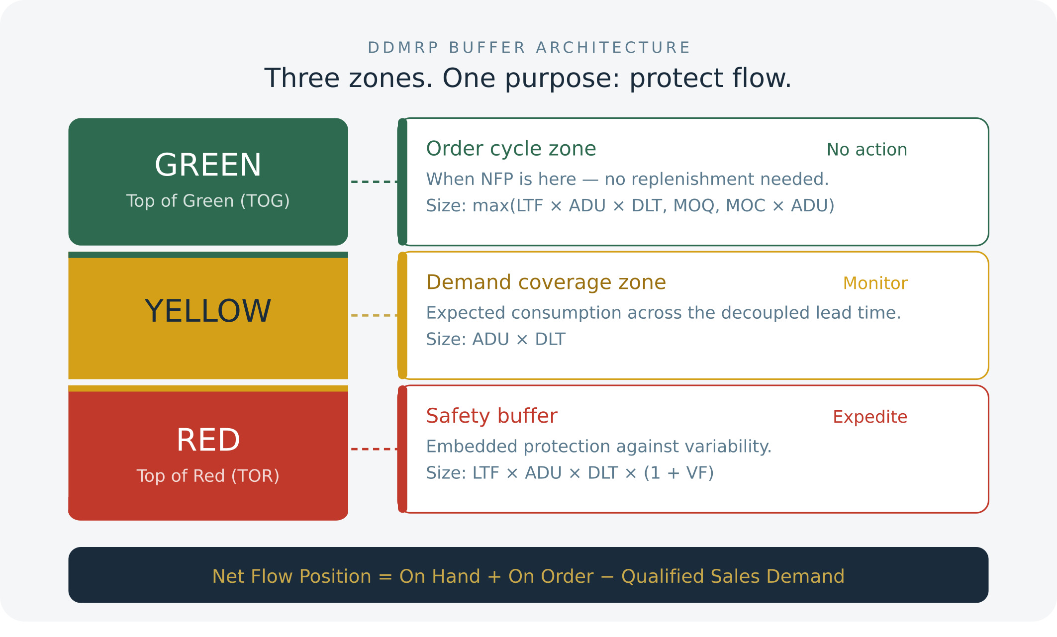
Variation is inevitable, whether it emerges from the market or from suppliers and production. The effective response is to assume it will be present and build compensating mechanisms that minimise the damage. A demand driven operating model uses three buffer types, each sized for a specific category of variation.
A material buffer sized from average daily usage, decoupled lead time and demand variability. Net flow position against these zones triggers replenishment, replacing the MRP run against forecast.
- Material buffers sit at strategic decoupling points, sized by average daily usage, decoupled lead time and demand variability. When demand spikes the buffer absorbs the surge while replenishment catches up. When demand falls, replenishment slows naturally and no excess accumulates. In engineer-to-order and make-to-order environments these typically cover core materials and long lead time components. In make-to-stock they cover finished goods and a majority of subordinate items.
- Time buffers sit in front of control points and strategic decoupling points on the shop floor. They ensure no production time is lost at the resource that constrains the entire flow, and they protect promise date performance by absorbing upstream supply and production variability. A work order arriving at the constraint inside its time buffer is not a crisis, it is the buffer doing its job. Penetration also gives visibility of upstream issues before they reach the constraint, and signals where improvement effort will pay.
- Capacity buffers are protected capacity at non-constraint resources, providing the sprint capability to recover from upstream variation without disrupting the constraint schedule. They look like unutilised capacity on a utilisation report. They are the mechanism that stops variation amplifying through the entire flow.
Counter-principle three · Reposition the forecast as a stress test
If replenishment is driven by actual consumption and variation is absorbed by buffers, what is the forecast for? Its role becomes evaluative rather than directive. The forecast feeds simulations of the operating model under expected demand. Will buffer configurations hold through a seasonal ramp? Will rough-cut capacity accommodate a promotional surge? Will time buffers protect promise dates?
The output is a diagnosis of where the model is at risk and the configuration changes needed in anticipation: buffers recalibrated, an item moved from a trailing to a forward-looking demand rate, an adjustment factor applied ahead of a seasonal peak, capacity expanded, a new product staged. The forecast is not used to drive committed orders. It tests whether the operating model can flex to the outcomes the business may face.
Roughly right, fed into a well-designed model, beats precisely wrong fed into a rigid plan.
The model in practice
The three principles fit together as a single operating system. Day to day, the model runs without forecast intervention. Buffers replenish automatically against actual consumption. Materials managers monitor buffer status and health rather than forecast accuracy. Production scheduling pulls from real demand. Exceptions are buffer status alerts: items penetrating their red zone, capacity buffers exhausted, time buffers consumed. The planner operates like a pilot on a commercial flight, not hand-flying the aircraft but monitoring conditions and intervening on an exception basis.
Periodically, as part of the demand driven S&OP cycle, one or more forecasts are fed into a simulation of the model under future-state scenarios. The simulation surfaces projected exposures: where buffers will fail, where capacity will strain, which items need a configuration change before the demand window arrives. Those changes are made in anticipation, not in reaction. The system then returns to consumption-paced operation until the next cycle.
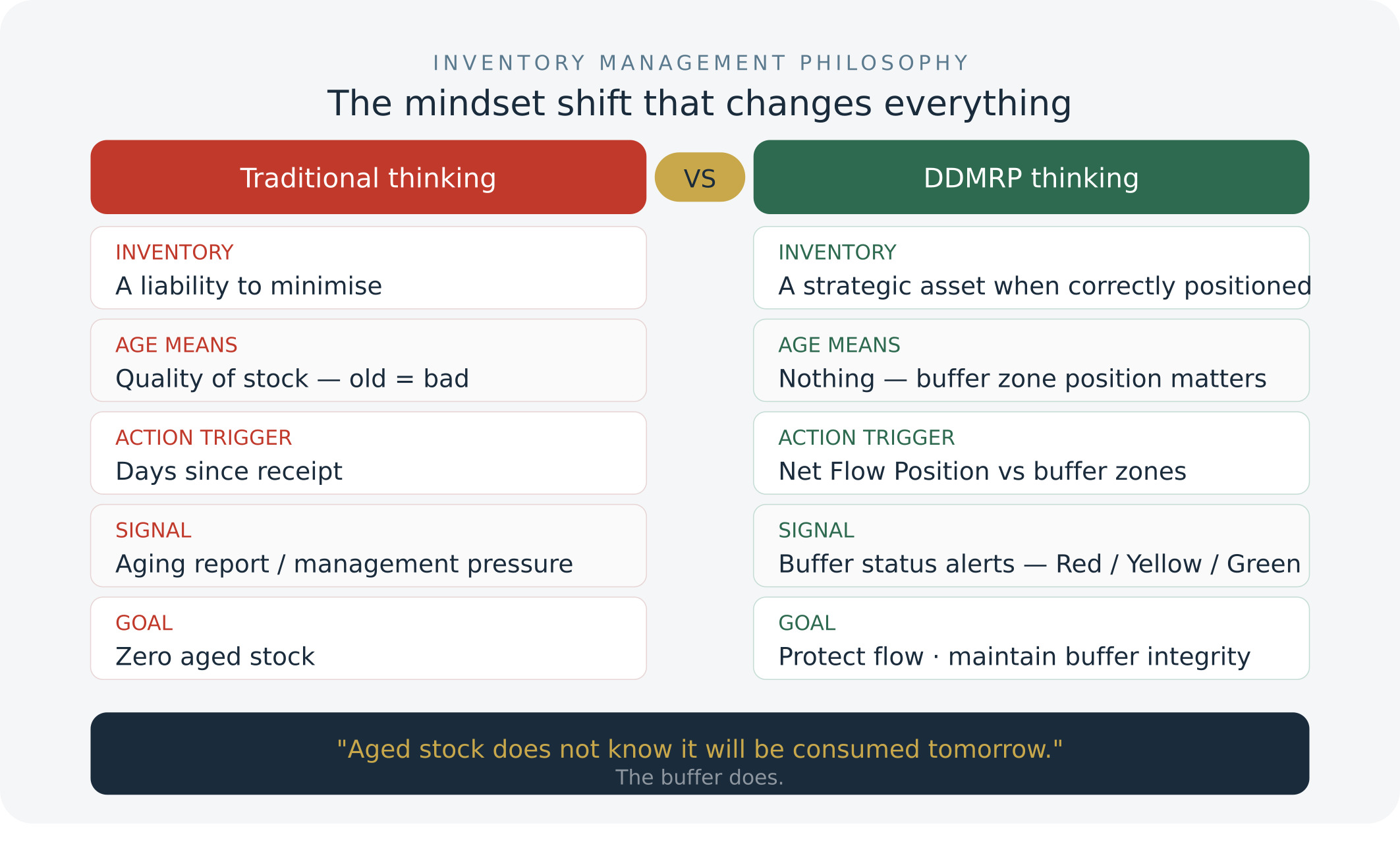
| Dimension | MRP-led model | Demand driven operating model |
|---|---|---|
| Demand signal | Forecast (predicted) | Actual consumption (observed) |
| Replenishment trigger | MRP run against forecast | Net flow position against buffer zones |
| Variation handling | Static or manually maintained safety stock | Strategic buffers sized for demand rate, lead time and variability |
| Forecast role | Drives the master production schedule | Stress test that informs buffer and capacity design |
| Planner role | Improve accuracy, expedite exceptions, pull in and push out | Configure and tune buffers, monitor model fitness |
| Demand surges | Forecast revised, supply chain whipsaws, expedite spend rises | Buffers flex upward and absorb the surge, replenishment accelerates |
| Demand falls | Excess accumulates, downward revisions rarely trigger drawdown | Buffers flex downward, replenishment slows, no excess builds |
| Working capital | Bloats over time and is hard to release | Sized to actual demand, released progressively as the model tunes |
| Service | Bimodal: stockouts and excess at the same time | High availability at lower carrying inventory |
MRP-led planning compared with a demand driven operating model across nine operating dimensions.
This is not a software upgrade. It is a redesign of how the supply chain operates.
Design the model deliberately
In a conventional planning organisation the operating model has accumulated rather than been engineered. The forecast drives replenishment because it always has. Safety stocks and safety lead times were inserted at points where service failed in the past and have not been questioned since. Lead times, sources of variation, decoupling points and risk-absorbing mechanisms have never been examined as a coherent whole. The result runs against assumptions nobody currently remembers making.
The first step of every successful deployment is not the installation of software. It is a deliberate step back with the leadership team to design the model itself. Where should the strategic stocking positions sit? Which production flows warrant time or capacity buffers? Where is variation entering the system, and which buffer type is best suited to absorb it? What are the actual lead times, and where does the planning system assume lead times that no longer hold?
That exercise is always revealing. Companies discover that master planning parameters are years out of date, that safety stocks are sized by rule of thumb rather than by any recognition of the demand patterns that exist, and that no one holds a documented rationale for how the model was set up. The design work is not a preface to the real implementation. It is the real implementation. Everything else is instrumentation.
Once the model has been designed, S&OP takes on a different role. Rather than a monthly reconciliation of forecast against reality, it becomes a continuous revision of the model itself. The question moves from what is our forecast accuracy to what is our adaptation capability, which the operating model can actually answer, and which produces action rather than argument.
Working capital is freed
Material buffers sized to actual demand and variability typically yield inventory reductions of twenty five to thirty five percent, broadly in line with the forecast inaccuracy the business is already absorbing. Capital previously trapped becomes available for capacity, debt reduction or growth.
Service improves
Because buffers are sized for variability rather than accuracy, items are available when consumption arrives, including the items that previously stocked out because the forecast missed them. The bimodal distribution resolves.
The firefight is retired
Planners stop chasing the forecast and stop reconciling the gap between plan and reality. Their work shifts to model configuration, buffer tuning and simulation, work that compounds rather than dissipating into next week’s exception queue. The job becomes a craft rather than a treadmill.
Where Kiira works
What changes when your ERP is Dynamics 365
Most of the literature on demand driven operating models is written as though the ERP underneath is a neutral container. It is not. The model has to be expressed in the system your planners log into every morning, and in a Dynamics 365 Finance and Operations environment that raises a specific set of questions we work through with every client.
- Lead time integrity. D365 master planning schedules backwards from the lead times held on the item and the default order settings, and treats them as deterministic. Where actual receipt performance diverges from the maintained lead time, the plan is wrong before it is published. Establishing true decoupled lead time, rather than inherited purchase lead time, is usually the highest-value data work in the engagement.
- Coverage codes and safety stock. Coverage groups, minimum and maximum keys and manually maintained safety stock journals are the accreted remains of past service failures. They need to be inventoried, rationalised, and then either retired or converted into buffer parameters with a documented rationale. Running buffer logic on top of an untouched safety stock layer double counts protection and inflates inventory.
- Where the buffer logic lives. The design decision is which items D365 continues to plan conventionally, which are governed by net flow against a buffer, and how supply recommendations flow back into D365 as planned orders without breaking approval, budget and procurement controls. This boundary determines whether planners trust the recommendation or quietly revert to the spreadsheet.
- Instrumentation. Intuiflow supplies the buffer engine, the net flow calculation, the execution alerts and the S&OP simulation layer. D365 remains the transactional system of record. Kiira designs and delivers both sides of that boundary, which is why operating model design and ERP configuration run as a single workstream rather than two projects that meet at a go-live date.
Why we position these together
A well-designed operating model implemented on an ERP configured against assumptions nobody remembers making will underperform. A beautifully configured ERP running forecast-led logic will keep producing exactly the results described in part one of this paper. The two have to move together.
For the agenda
Five questions for the board
Most demand planning conversations never reach the board. They are treated as operational hygiene, line items in a supply chain budget, or vendor decisions delegated to IT. That framing understates the stakes. A company carrying twenty percent more inventory than it needs is funding that excess with working capital that could service growth, return to shareholders or absorb a downturn.
- What is the marginal return on our next rand invested in forecast accuracy? If management cannot answer in working capital or service level terms, the programme has no stopping rule and is almost certainly past the point of diminishing returns.
- Where on the spectrum from make-to-order to make-to-stock does our business actually sit, and is our planning approach matched to it? Forecast-led planning in a high velocity, high variability environment is the most common and most expensive misalignment in supply chain operations.
- How much of our planning effort is concentrated on the items that drive a meaningful share of revenue? Pareto routinely shows a small percentage of items generating eighty to ninety percent of revenue, while planning attention is spread evenly across the long tail.
- Are we trapped in customisation? Heavily customised platforms narrow the field of vision to the company’s own past practices and lock out external innovation. The spend is rarely visible at board level. The strategic cost is significant.
- If we released ten percent of our inventory, what would we do with the capital? If the answer is unclear, this is not yet a board priority. If it is concrete, whether capacity expansion, debt reduction, acquisition capacity or dividend support, the conversation belongs on the agenda.
The capital allocation lens
The temptation, when supply chain performance disappoints, is to buy a better forecasting system, hire more planners or commission another transformation. Each is defensible in isolation. None of them, on the evidence of the last thirty years, will materially change the inventory-to-sales ratio of a typical manufacturer or distributor.
What will change it is a deliberate decision, made where capital allocation decisions are made, to shift the operating model from forecast-led to demand driven, to accept that forecasts will remain imperfect, and to invest the savings in resilience and growth rather than in chasing accuracy the data will never deliver.
The prize is not a better forecast. It is the capital that better forecasts have failed to release.
About Kiira Consulting
Clarity, capability and long-term operational excellence
Kiira Consulting is a Microsoft Dynamics 365 Finance and Operations and demand driven supply chain transformation partner based in Johannesburg. We design, implement and optimise high-performance digital operations by aligning technology, process and people to support stable, agile and flow-driven performance.
Our team brings decades of combined expertise across ERP architecture, solution design, technical delivery and continuous improvement. Beyond ERP capability we specialise in demand driven methodologies including DDMRP, DDOM and flow-based planning, enabling organisations to reduce noise, improve visibility, stabilise planning environments and build resilient, adaptive supply chains.
Next step
The diagnostic in part two is the fastest way to establish whether this argument applies to your business. Kiira runs it as a structured assessment against your own forecast history and inventory position, and delivers the result as a board-ready view of where your operating model is costing you capital. If the variability ranges come back below thirty points, we will tell you so.
This article consolidates and adapts material from a four-part series on supply chain operating model design authored by Erik Bush, published by Kiira Consulting with permission. The methodology draws on the Demand Driven Institute body of knowledge, including DDMRP, DDOM and DDS&OP, and on the theory of constraints and lean traditions from which it derives. Intuiflow is a product of Demand Driven Technologies. Figures and thresholds are illustrative and should be replaced with client data before internal use.
© Kiira Consulting · Johannesburg, South Africa